This documentation is availlable online at https://fvigneron.github.io/FastPolyEval. It also exists in PDF form: FastPolyEval_doc.pdf. The source code can be found on GitHub.

Abstract

FastPolyEval is a library, written in C, that aims at evaluating polynomials very efficiently, without compromising the accuracy of the result. It is based on the FPE algorithm (Fast Polynomial Evaluator) introduced in reference [1] (see Section References, Contacts and Copyright).

In FastPolyEval, the computations are done for real or complex numbers, in floating point arithmetic, with a fixed precision, which can be one of the machine types FP32, FP64, FP80 or an arbitrary precision based on MPFR.

Evaluations are performed on arbitrary (finite...) sets of points in the complex plane or along the real line, without geometrical constraints.

The average speed-up achieved by FastPolyEval over Hörner's scheme is illustrated on Figure 1.

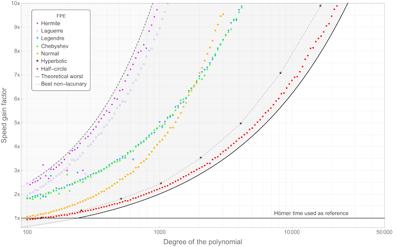
Figure 1: Speed gain of FastPolyEval versus Hörner for O(d) evaluations in precision p=53 MPFR.

Complexity & accuracy

FastPolyEval splits the evaluation process in two phases:

A first phase, called pre-processing, analyses the coefficients of the polynomial (actually only the exponents) and determines an evaluator, based on a parcimonious representation of the polynomial.
Subsequently, the evaluator is applied to each of the requested evaluation points. A second reduction is performed. Then the final result is computed.

The complexity of the pre-processing phase is bounded by $ O(d \log d)$ where $ d$ is the degree of the polynomial $ P(z)$. It is independent of the precision used to express the coefficients or requested for the rest of the computations. The FastPolyEval library is backed by theoretical results that guaranty that the average arithmetic complexity of the final evaluator is of order

\[ O\left( \sqrt{d(p+\log d)} \right) \]

where $ p$ is the precision of the computation, in bits. The averaging process corresponds to evaluation points $ z$ uniformly distributed either on the Riemann sphere or on the unit disk of the complex plane. The worst complexity of the evaluator does not exceed that of Hörner, i.e. $ O(d)$, and can drop as low as $ O(\log^2 d)$ in some favorable cases (see Figure 1 in Abstract).

The memory requirement of FastPolyEval is minimal. To handle a polynomial of degre $ d$ with $ p$ bits of precision, the memory requirement is $ O(dp)$. An additional memory $ O(kp)$ is required to perform $ k$ evaluations in one call.

Regarding accuracy, the theory guaranties that the relative error between the exact value of $ P(z)$ and the computed value does not exced $ 2^{-p-c-1}$ where $ c$ is the number of cancelled leading bits, i.e.

\[ c = \begin{cases} 0 & \text{if } |P(z)| \geq M(z),\\ \left\lfloor \log_2\left| M(z) \right| \right\rfloor - \left\lfloor \log_2\left| P(z) \right| \right\rfloor & \text{else,} \end{cases} \]

where $ M(z)=\max |a_j z^j|$ is the maximum modulus of the monomials of $ P(z)$ and $ \lfloor\cdot\rfloor$ is the floor function.

Note: The geometric preprocessing uses only the exponents of the coefficients, which is a significantly smaller amount of data to process than reading all the bits of the coefficients. For a high-precision high-degree evaluation at a single point, FastPolyEval can often outperform Hörner. The preprocessing of the exponents followed by the evaluation with a high precision of a parcimonious representation of the polynomial is more efficient than handling indiscriminately all the coefficients. This fact does not contradict that Hörner is a theoretical best for one single evaluation. Hörner has the best estimate on complexity that holds for any evaluation point. The advantage of FastPolyEval can be substantial, but it holds on average. Note that the worst case for the evaluator (no coefficient dropped) has the same complexity as Hörner. However, in that case, one can prove that the average complexity is much better, typicaly $ O(\log^2 d) $.

For further details, precise statements and proofs, please see reference [1] in section References, Contacts and Copyright.

Description of the Fast Polynomial Evaluator (FPE) algorithm

In this section, we describe briefly the mathematical principles at the foundation of FastPolyEval.

General principles

FastPolyEval relies on two general principles.

Lazy evaluation in finite precision. When adding two floating points numbers with p bits, one can simply discard the smaller one if the orders of magnitude are so far apart that the leading bit of the smaller number cannot affect the bit in the last position of the larger number. When evaluating a polynomial of large degree, the orders of magnitude of the monomials tends to be extremely varied, which is a strong incentive to use lazy evaluations.
Geometric selection principle. For a given evaluation point, evaluating each monomial and sorting them in decreasing order of magnitude would be a very inefficient way of implementing lazy additions. Instead, FastPolyEval can identify the leading monomials using a simple geometric method that allows us to factor most of the work in a pre-processing phase, which is only needed once. At each evaluation point, a subsequent reduction produces a very parcimonious representation of the polynomial (see Figure 2).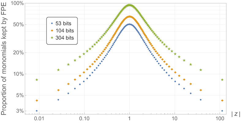

Figure 2: Parsimony of the representation used by FastPolyEval to evaluate a polynomial of degree 1000 (half-circle family).

Geometric selection principle

For a given polynomial $ P$ of degree $ d$, one represents the modulus of the coefficients $ a_j$ in logarithmic coordinates, that is the scatter plot $ E_P$ of $ \log_2 |a_j|$ in function of $ j\in \{0,1,\ldots,d\}$. One then computes the concave envelope $ \hat{E}_P$ of $ E_P$ (obviously piecewise linear) and one identifies the strip $ S_\delta(\hat{E}_P)$ situated below $ \hat{E}_P$ and of vertical thickness

\[ \delta = p + \lfloor \log_2 d \rfloor + 4. \]

Note that the thickness of this strip is mostly driven by the precision $ p$ (in bits) that will be used to evaluate $ P$. On Figure 3, the blue points represent $ E_P$, the cyan line is $ \hat{E}_P$ and the strip $ S_\delta$ is colored in light pink.

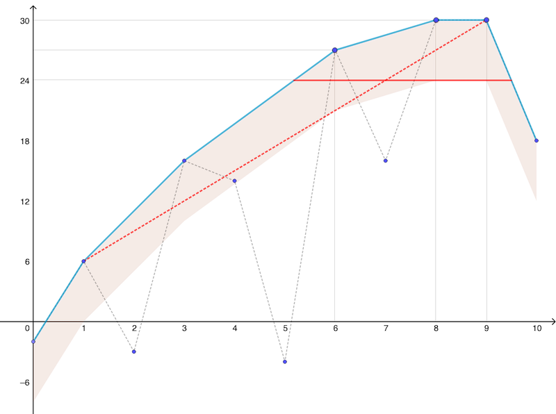
Figure 3: Concave cover of the oefficients of a polynomial (log-scale) and selection principle for a given precision.

The coefficients of $ P$ that lie in the strip $ S_\delta$ are pertinent for an evaluation with precision $ p$. The others can safely be discarded because they will never be used at this precision.

Parcimonious representation at an arbitrary point

For a given $ z\in\mathbb{C}$, a parcimonious representation of $ P(z)=\sum\limits_{j=0}^d a_j z^j$ is obtained by selecting a proper subset of the indices $ J_p(z) \subset\{0,1,\ldots,d\}$ and discarding the other monomials:

\[ Q_p(z) = \sum_{j\in J_p(z)} a_j z^j. \]

For computations with a precision of $ p$ bits, the values of $ Q_p(z)$ and $ P(z)$ are equivalent because the relative error does not exceed $ 2^{-p-c-1}$ where c is the number of cancelled leading bits (defined in Section Complexity & accuracy).

The subset $ J_p(z)$ is obtained as a subset of the (indices of the) coefficients that respect the two following criteria in the logarithmic representation (see Figure 3):

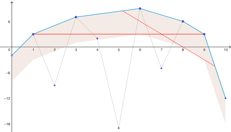
the coefficient belongs to the strip $ S_\delta$,
the coefficient is above the longest segment of slope $ \tan\theta = -\log_2|z| $ contained in $ S_\delta$.

The selecting segment is always tangent to the lower edge of $ S_\delta$ or, in case of ambiguity (e.g. if $ S_\delta$ is a parallelogram), it is required to be. For $ |z|=1$, the selecting segment is an horizontal line illustrated in solid red in Figure 3 above. The red dashed line corresponds to some value $ |z|<1$. Figure 4 illustrates how the selection principle at an arbitrary point $ z\in\mathbb{C}$ can be transposed from the analysis performed on the raw coefficients, i.e. for $ |z|=1$. In log-coordinates, one has indeed: $ \log_2\left( |a_j z^j | \right) = \log_2 |a_j| - j \tan\theta.$ Selecting the coefficients such that $ \log_2\left( |a_j z^j | \right)$ differs from its maximum value by less than $ \delta$ (solid red in Figure 4) is equivalent to selecting those above the segment of slope $ \tan\theta$ in the original configuration (dashed line in Figure 3).

Figure 4: Transposition of the selection principle at an arbitrary evaluation point

Implementation of the algorithm

FastPolyEval computes Figure 3 and the strip $ S_\delta$ in the pre-processing phase and keeps only the subset of the coefficients that belong to that strip (the so-called "good" set $ G_p$ in reference [1]). In the evaluation phase, the subset of coefficients is thinned to $ J_p(z)$ for each evaluation point $ z$ using the 2nd criterion, thus providing the parcimonious representation $ Q_p(z)$ of $ P(z)$ at that point. The value of the polynomial is then computed using Hörner's method for $ Q_p$. Theoretical results guaranty that, on average, the number of coefficients kept in $ J_p(z)$ is only of order $ \sqrt{d \delta}$, which explains why the complexity of FastPolyEval is so advantageous.

For further details, see reference [1] in Section References, Contacts and Copyright.

Installation of FastPolyEval

FastPolyEval is distributed as source code, written in the C language. The source code can be downloaded from our public github repository.

Prerequisites

First of all, don't panic, it's easy...

Obvioulsy, you will need a computer and a C compiler, for example GCC, though any other C compiler will be fine.

FastPolyEval relies on MPFR to handle floating point numbers with arbitrary precision. You need to install this library on your system if it is not already installed. Please follow the MPFR installation instructions to do so. Note that MPFR has one main depency, GMP, which will also need to be installed (see the GMP installation instructions). If you do not have admin privileges on your machine, you can still build those libraries in a local directory and instruct your compiler to look for the appropriate library path. For example, if you use GCC, see the documentation of option -L.

Note that on most OS, one can also install those libraries through a package manager (see Additional help for Linux, MacOS, Windows).

Note: The libraries GMP and MPFR are free to download and use and are distributed under the Lesser General Public License, which enables developers of non-free programs to use GMP/MPFR in their programs. FastPolyEval is released under the BSD licence, with an attribution clause (see References, Contacts and Copyright), which means that you are free to download, use, modify, distribute or sell, provided you give us proper credit.

Compile FastPolyEval

Download the source code. In the command line, go to the code subfolder then type:

make

to get a basic help message. The default build command is:

make fpe

This will create and populate a bin subdirectory of the downloaded folder with an app, called FastPolyEval. You may move the executable file to a convenient location. Alternatively, consider adding this folder to your PATH. The Makefile does not attempt this step for you. See Basic usage of FastPolyEval for additional help on how to use this app.

If you prefer to compile by hand, the structure of your command line should be:

gcc all_source_files.c -o bin/FastPolyEval -I each_source_sub_folder_containing_header_files -Wall -lm -lgmp -lmpfr -O3

Note that the file.c and -I folder parameters must be repeated as necessary. The Makefile is simple enough and understanding it can provide additional guidance.

FastPolyEval switches automatically from hardware machine precision to emulated high-precision using MPFR (see Number formats). The format used for hardware numbers is chosen at the time of the compilation. You may edit the source file code/numbers/ntypes.h before the default build. Alternatively, you can execute

make hardware

This should generate an automatically edited copy of this header file in a temporary folder and launch successive compilations. This build will populate the bin subdirectory with three apps, called FastPolyEval_FP32, FastPolyEval_FP64 and FastPolyEval_FP80 corresponding to each possible choice.

Additional help for Linux, MacOS, Windows

Github offers access to virtual machines that run on their servers. The corresponding tasks are called workflows. Each workflow serves as a guidline (read the subsection job:steps in the yml files) to perform similar actions on your computer. The directory .github/workflows on our GitHub repository contains a build workflow for each major OS : Linux, MacOS and Windows.

Uninstall FastPolyEval

As the Makefile does not move the binaries and does not alter your PATH, cleanup is minimal. To remove the binary files generated in the build process, execute

make clean

To uninstall FastPolyEval from your system, simply delete the executable file and remove the downloaded sources.

Basic usage of FastPolyEval

FastPolyEval is used at the command line, either directly or through a shell script. A typical command line call has the following structure:

FastPolyEval -task prec parameter [optional_parameter]

where prec is the requested precision for the computations.

Onboard help system

To call the onboard help with a list and brief description of all possible tasks, type

FastPolyEval -help

help_struct

Description of a basic help screen.

Definition: help.h:73

A detailed help exists for each task. For example, try FastPolyEval -eval -help.

The different tasks belong to 3 groups:

and will be detailed below.

Note: In absence of argument, the default behavior is a call for help. The previous messaged can also be displayed respectively with FastPolyEval and FastPolyEval -eval .

Number formats

The flags MACHINE_LOW_PREC and MACHINE_EXTRA_PREC in ntypes.h define what kind of machine numbers FastPolyEval defaults to for low-precision computations, and the corresponding precision threshold that defines how low is "low". Note that the main limitation of machine numbers is the limited range of exponents. The numerical limits can easily be reached when evaluating a polynomial of high degree. On the contrary, MPFR number are virtually unlimited, with a default ceiling set to $ \simeq 2^{\pm 4\times 10^{18}}$.

Number formats
`numbers/ntypes.h`	Precision requested	Format	Numerical limit
MACHINE_LOW_PREC	up to 24	FP32, `float`	about $ 10^{-38}$ to $ 10^{+ 38}$
MACHINE_LOW_PREC	25 and up	MPFR	practically unlimited
no flag	up to 53	FP64, `double`	about $ 10^{- 308}$ to $ 10^{+ 308}$
no flag	54 and up	MPFR	practically unlimited
MACHINE_EXTRA_PREC	up to 64	FP80, `long` `double`	about $ 10^{- 4930}$ to $ 10^{+ 4930}$
MACHINE_EXTRA_PREC	65 and up	MPFR	practically unlimited

Warning: If a number either read as input from a file or computed and destined to the output cannot be represented with the selected precision (inf or NaN exception), a warning is issued and the operation fails. Usually, the solution consists in using a higher precision (i.e. MPFR numbers). Anoter possible issue (if you are running Newton steps) is that you have entered the immediate neigborhood of a critical point, which induces a division by zero or almost zero. Try neutralizing the offending point.

Other numerical settings can be adjusted in ntypes.h, in particular :

HUGE_DEGREES sets the highest polynomial degree that can be handled (default $ 2^{64}-2$),
HUGE_MP_EXP sets the highest exponent that MPFR numbers can handle (default $ \pm 4 \times 10^{18} $).

Input and outputs

FastPolyEval reads its input data from files and produces its output as file. The file format is CSV. To be valid, the rest of the CSV must contains a listing of complex numbers, written

a, b

where a is the real part and b is the imaginary part, in decimal form.

Depending on the context, the file will be interpreted as a set of evaluation points, a set of values, or the coefficients of a polynomial. For example, here is a valid file:

// An approximation of pi
3.14, 0
// A complex number close to the real axis
1.89755593218329076e+99, 2.35849881747969046e-427

Polynomials are written with the lowest degree first, so $ P(z) = 1-2 i z$ is represented by the file

1, 0

0, -2

Comments line are allowed: they start either with #, // or ;. Comment lines will be ignored. Be mindful of the fact that comments can induce an offset between the line count of the file and the internal line count of FastPolyEval. Blank lines are not allowed. Lines are limited to 10 000 symbols (see array_read), which puts a practical limit to the precision at around 15 000 bits. You can easily edit the code to push this limitation if you have the need for it.

Warning: As a general rule for the tasks of FastPolyEval, if an output file name matches the one of an input file, the operation is safe. However, the desired output will overwrite the previous version of the file.

Note: For users that want a turnkey solution to high-performance polynomial evaluations where the outputs of some computations are fed back as input to others, we recommend the use of FastPolyEval with data residing in a virtual RAM disk, on local solid-state drives or on similar low latency/high bandwidth storage solutions. If you have doubts on how to do this, please contact your system administrator.

Tasks for generating and handling polynomials

FastPolyEval contains a comprehensive set of tools to generate new polynomials, either from scratch or by performing simple operations on other ones.

Classical polynomials are generated with the tasks -Chebyshev, -Legendre, -Hermite, -Laguerre. The family -hyperbolic is defined recursively by
\[ p_1(z)=z, \qquad p_{n+1}(z) = p_n(z)^2 + z \]
and plays a central role in the study of the Mandelbrot set (see e.g. reference [2] in References, Contacts and Copyright).
One can build a polynomial from a predetermined set of roots (listed with multiplicity) by invoquing the task -roots.
One can compute the sum (-sum), difference (-diff), product (-prod) or the derivative (-der) of polynomials.

Tasks for generating and handling sets of complex numbers

FastPolyEval contains a comprehensive set of tools to generate new sets of real and complex numbers, either from scratch or by performing simple operations on other ones.

The real (-re) and imaginary (-im) parts of a list of complex numbers can be extracted. The results are real and therefore of the form x, 0 . The complex conjugate (sign change of the imaginary part) is computed with -conj and the complex exponential with -exp.
FastPolyEval can perform various interactions between valid CSV files.
1. The concatenation (-cat) of two files writes a copy of the second one after a copy of the first one. For example, to rewrite a high-precision output file_high_prec.csv with a lower precision prec, use
  FastPolyEval prec file_high_prec.csv /dev/null file_low_prec.csv
2. The -join task takes the real parts of two sequences and builds a complex number out of it. The imaginary parts are lost.
```
     a, *    (entry k from file_1)
     b, *    (entry k from file_2)
     ----
     a, b    (output k)
```
  If the files have unequal lengh, the operation succeeds but stops once the shortest file runs out of entries. Be mindfull of offsets induced by commented lines (see Input and outputs).
3. The -tensor task computes a tensor product (i.e. complex multiplication line by line).
```
     a, b    (entry k from file_1)
     c, d    (entry k from file_2)
     ----
     ac-bd, ad+bc  (output k)
```
  If the files have unequal lengh, the operation succeeds but stops once the shortest file runs out of entries. Be mindfull of offsets induced by commented lines (see Input and outputs).
4. The -grid task computes the grid product of the real part of the entries. The output file contains nb_lines_file_1 $ \times$ nb_lines_file_2 lines and lists all the products possibles between the real part of entries in the first file with the real part of entries in the second file. The imaginary parts are ignored.
Rotations (-rot) map the complex number $ a + i b$ to $ a \times e^{i b}$. For example, to generate complex values from a real profile profile.csv and a set of phases phases.csv, you can use
FastPolyEval -join prec profile.csv phases.csv rot_tmp.csv

FastPolyEval -rot prec rot_tmp.csv complex_output.csv

rm -f rot_tmp.csv
The -unif task writes real numbers in an arithmetic progression whose characteristics are specified by the parameters.
The -sphere task writes polar coordinates approximating an uniform distribution on the Riemann sphere. The output value $ (a, b)$ represents Euler angles in the (vertical, horizontal) convention. It represents the point
\[ (\cos a \cos b, \cos a \sin b, \sin a) \in \mathbb{S}^2 \subset \mathbb{R}^3. \]
The -polar task maps a pair of (vertical, horizontal) angles onto the complex plane by stereographical projection. To generate complex points that are uniformly distributed on the Riemann sphere, starting with SEED points at the equator, you can use the following code that combines those tasks. Note that there will be about $ SEED^2/\pi$ points on the sphere and that the points are computed in a deterministic way (they will be identical from one call to the next). A SEED of 178 produces about 10 000 complex points.
SEED=178

FastPolyEval -sphere prec $SEED tmp_file.csv

FastPolyEval -polar prec tmp_file.csv sphere.csv

rm -f tmp_file.csv
FastPolyEval also contains two random generators (actually based on MPFR). The -rand task produces real random numbers that are uniformly distributed in an interval. The -normal task produces real random numbers with a Gaussian distribution whose characteristics are specified by the parameters. Use the -join task to merge the outputs of two -normal tasks into a complex valued normal distribution.

Tasks using the FPE algorithm for production use and benchmarking

The main tasks of the FastPolyEval library are the following:

-eval evaluates a polynomial on a set of points using the FPE algorithm.
-evalD evaluates the derivative of a polynomial on a set of points using the FPE algorithm.

The precision of the computation and the name of the inputs (polynomial and points) & output (values) files are given as parameters. The first optional parameter specifies a second output file that contains a complementary report on the estimated quality of the evaluation at the precision chosen. For each evaluation point, this report contains an upper bound for the evaluation errors (in bits), a conservative estimate on the number of correct bits of the result, and the number of terms that where kept by the FPE algorithm.

For benchmark purposes (see reference [1] in Section References, Contacts and Copyright), we propose a set of optional parameters that specify how many times the preprocessing and the FPE algorithm should be run at each point (to improve the accuracy of the time measurement), whether the Hörner algorithm should also be run and, if so, how many times it should run.

The task -evalN evaluates one Newton step of a polynomial on a set of points, i.e.

\[ \textrm{NS}(P,z) = \frac{P(z)}{P'(z)}. \]

Recall that Newton's method for finding roots of $ P$ consists in computing the sequence defined recursively by

\[ z_{n+1} = z_n -\textrm{NS}(P,z_n). \]

The -iterN task iterates the Newton method a certain amount of times and with a given precision. It thus realizes a partial search of the roots of the polynomial. For best results, we recommend successive calls where the precision is gradually increased and the maximum number of iterations is reduced. For guidance in the choice of the starting points, please refer to reference [3] in Section References, Contacts and Copyright.

-analyse computes the concave cover and the intervals of |z| for which the evaluation strategy changes

The -analyse task computes the concave cover $ \hat{E}_P$ , the strip $ S_\delta$ (see Section Description of the Fast Polynomial Evaluator (FPE) algorithm) and the intervals of |z| for which the evaluation strategy of FPE (i.e. the reduced polynomial $ Q_p(z)$) changes. It is intended mostly for an illustrative purpose on low degrees, when the internals of the FPE algorithm can still be checked by hand. However, the intervals where a parsimonious representation is valid may also be of practical use (see reference [1] in Section References, Contacts and Copyright).

Notes about the implementation

For further details, please read the documentation associated to each source file.

Do not hesitate to contact us (see References, Contacts and Copyright) to signal bugs and to request new features. We are happy to help the development of the community of the users of FastPolyEval.

References, Contacts and Copyright

Please cite the reference [1] below if you use or distribute this software. The other citations are in order of appearance in the text:

[1] R. Anton, N. Mihalache & F. Vigneron. Fast evaluation of real and complex polynomials. 2022. [hal-03820369].
[2] N. Mihalache & F. Vigneron. How to split a tera-polynomial. In preparation.
[3] J.H. Hubbard, D. Schleicher, S. Sutherland. How to find all roots of complex polynomials by Newton's method. Invent. math., 146:1-33, 2001. [Llink] on author's page.

Authors: Nicolae Mihalache – Université Paris-Est Créteil (nicol.nosp@m.ae.m.nosp@m.ihala.nosp@m.che@.nosp@m.u-pec.nosp@m..fr)
François Vigneron – Université de Reims Champagne-Ardenne (franc.nosp@m.ois..nosp@m.vigne.nosp@m.ron@.nosp@m.univ-.nosp@m.reim.nosp@m.s.fr)

Copyright: This software is released under the BSD licence, with an attribution clause (see License).
Copyright 2022 – Université Paris-Est Créteil & Université de Reims Champagne-Ardenne.

Thanks

It is our pleasure to thank our families who supported us in the long and, at times stressful, process that gave birth to the FastPolyEval library, in particular Ramona who co-authored reference [1], Sarah for a thorough proof-reading of [1] and Anna who suggested the lightning pattern for our logo.

We also thank Romeo, the HPC center of the University of Reims Champagne-Ardenne, on which we where able to benchmark our code graciously.

License

Redistribution and use in source and binary forms, with or without modification, are permitted provided that the following conditions are met:

Redistributions of source code must retain the above copyright notice, this list of conditions and the following disclaimer.
Redistributions in binary form must reproduce the above copyright notice, this list of conditions and the following disclaimer in the documentation and/or other materials provided with the distribution.
Neither the name of the copyright holder nor the names of its contributors may be used to endorse or promote products derived from this software without specific prior written permission.
Redistributions of any form whatsoever must retain the following acknowledgment:

'This product includes software developed by Nicolae Mihalache & François Vigneron at Univ. Paris-Est Créteil & Univ. de Reims Champagne-Ardenne. Please cite the following reference if you use or distribute this software: R. Anton, N. Mihalache & F. Vigneron. Fast evaluation of real and complex polynomials. 2022. [arxiv-2211.06320] or [hal-03820369]'

THIS SOFTWARE IS PROVIDED BY THE COPYRIGHT HOLDERS AND CONTRIBUTORS "AS IS" AND ANY EXPRESS OR IMPLIED WARRANTIES, INCLUDING, BUT NOT LIMITED TO, THE IMPLIED WARRANTIES OF MERCHANTABILITY AND FITNESS FOR A PARTICULAR PURPOSE ARE DISCLAIMED. IN NO EVENT SHALL THE COPYRIGHT HOLDER OR CONTRIBUTORS BE LIABLE FOR ANY DIRECT, INDIRECT, INCIDENTAL, SPECIAL, EXEMPLARY, OR CONSEQUENTIAL DAMAGES (INCLUDING, BUT NOT LIMITED TO, PROCUREMENT OF SUBSTITUTE GOODS OR SERVICES; LOSS OF USE, DATA, OR PROFITS; OR BUSINESS INTERRUPTION) HOWEVER CAUSED AND ON ANY THEORY OF LIABILITY, WHETHER IN CONTRACT, STRICT LIABILITY, OR TORT (INCLUDING NEGLIGENCE OR OTHERWISE) ARISING IN ANY WAY OUT OF THE USE OF THIS SOFTWARE, EVEN IF ADVISED OF THE POSSIBILITY OF SUCH DAMAGE.

Table of Contents